Microsoft Excel. Love it or hate it, but chances are if you’re in this digital marketing industry of ours, it plays an integral part in your daily working routine. Indeed, if you’re anything like me (and I sit firmly in the love category by the way) you spend an enormous % of your day working with it in some capacity or another. With this in mind, I’ve decided to present some small tips and tricks that I’ve picked up over the years that may just save your life! (Well, at least save you a lot of time and effort in the long-run..)
Before we delve into these life saving tips, I ought to mention that if you’re a more advanced user you may enjoy Found’s latest Excel cheat sheet with 43 useful formulas and a series of powerful macros thrown in for good measure. It’s aimed at digital marketers but there’s plenty there for anyone. Now, back to our top tips..
1. Multiple Insert / Multiple Delete
This first point is a classic example of a tiny tip saving a huge amount of time. I won’t name names, but a few months back I stumbled across a colleague who asked me if there was a quick way to insert many rows in his worksheet. He had already populated his worksheet with a lot of data, but found that he wanted to clear a big space in the middle of it (about 100 rows). So his approach was to add in single rows… 100 times over!
So the way in which he was doing this was to right click on the numbers down the left-hand side, and then clicking on ‘insert’. One row will appear in-between. Useful, yes, but not for mass amounts of rows. In order to insert multiple rows, you have several options:
a) Highlight (drag your mouse) over many of these numbers, then right click, then ‘insert’.
b) Highlight a range of rows in your table, right click, ‘insert’, then ‘shift cells down’.
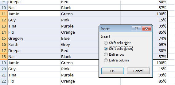
The first option will add the rows across the whole worksheet, whereas the second option will just do it for that table. Why not try it at home now?
Best used: When you want to add or delete lots of data from the middle of a worksheet.
2. Open Excel on two screens at once
If you’re a smug media-type like me, you may make use of multiple screens at once – casually checking twitter trends on one screen whilst triumphantly SUMIF’ing on the other. But what if you want to compare two Excel sheets at once, and constantly switching sheets on one monitor is really starting to do your head in?
Well fear not, for there is a way!
Essentially all you need to do is open Excel again (I know, easy right?). Chances are if you have multiple Excel sheets open at the same time, they’re all bound to the same instance of the program, so when you switch between them they appear on the same screen as all the others. To open a new instance simply re-open Excel anew, from scratch (either by double clicking on your desktop icon or by loading it from your start bar). Drag this second instance across to your other screen and voila!
Best Used: When you want to compare things quickly side by side.
3. The Format Painter is your friend
Have you ever found yourself trying to replicate a certain style or format several times over, and spent ages messing around with all the colours and fonts? Have you ever tried to replicate a custom colour and spent ages searching through the colour palette to try and get it ‘just right’?
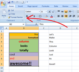
The format painter is a great little tool that allows you to select any cell or set of cells, and copy all formatting from them into new ones. You can locate it at the top left of your tool bar. Simply highlight the cells with the formatting that you want to copy and click on ‘format painter’. A little paintbrush icon will appear – then dragging this over other cells will copy the formatting into them.
But wait, think you know the format painter already? Here’s another tip for free:
When you want to copy a set of formatted cells multiple times, you can! Rather than clicking on ‘format painter’ once, double click it instead. You can run it over a set of cells multiple times without it resetting – a handy little timesaver that one!
Best Used: Particularly useful when you’re trying to replicate a custom colour, and would otherwise have to trawl through and replicate by trial and error.
4. Who needs a mouse?
Remember these keys, and remember them well. Ctrl. Shift. Up. Down. Left. Right.
Fast navigation in Excel is perhaps the best thing ever invented, and is the one thing that has single-handedly saved me the most time over the course of my Excel ‘career’. I first discovered it way back in Year 7 IT class, when we would gleefully sabotage mate’s spreadsheets when they weren’t looking – quickly navigating to the far bottom right of their worksheet and writing the word ‘bum’, before quickly shooting back up to the top again. What crazy times!
Nowadays I use it to navigate around Excel sheets at lightning fast speed. Using the arrow keys will move your selector across the cells, but if you use Ctrl at the same time, it can do two things:
1) If you’re in the middle of a selection of data, it will shoot you to the end of that data, in any direction. If you’re on record 10 of 5000 for instance, using Ctrl and the down arrow at the same time will shoot you all the way down to record 5000 instantly.
2) If you’re on a blank cell, using this technique will move your cursor to the next non-empty cell in any direction.
Shift is also a very useful tool when used in conjunction with the arrow keys. Holding it down will allow you to highlight cells that you navigate across, allowing for rapid-fast cell selection. Using Ctrl, Shift and the arrow keys together allows you to select huge swathes of data in one fell swoop.
When you start to combine these tips with the other Ctrl shortcuts (such as copy and paste) it starts to become a lot more powerful, and believe me, will save you a hell of a lot of time!
Best used: When you’re trying to find the end of a particularly long list of data. When used in conjunction with other common shortcuts such as copy/cut and paste.
5. Using Find/Replace for fun & profit
Chances are you’re aware of the find function (or CTRL+F to the savvy user). Most programs have one, from spreadsheets, to word processers and internet browsers. It enables you to quickly skip to the data you want to find, best used when there’s a lot of data to hand. For instance I use it to quickly skip to my favourite Ricky Martin lyrics from his fanpage important business data in Excel.
You may even be aware of the find and replace function (or CTRL+H to the savvy user).
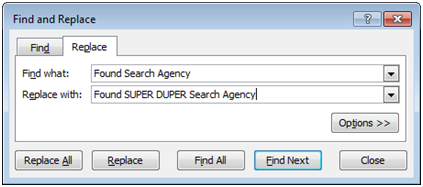
This can be used in lots of different ways, all of which can save you time. Some examples include:
- You’ve created a huge spreadsheet with lots of employee data but have accidentally misspelled the MD’s name 5000 times over (uh-oh!) Find/Replace: “Tnia” with “Tina”. 5000 records modified.
- You’ve been generating thousands of keywords for blue dresses on a fashion website. You want to move on to the next section, green, but don’t want to type out all of those keywords again. Copy the list, paste into a new column, find and replace “blue” with “green”.
- You’re trying to access commission references from a report, but it’s full of additional code:
<>Useful<tracking code>Information<tracking code>In<tracking code>Here<>
First: Find/Replace <> with [nothing]
Second: Find/Replace <tracking code> with [space]
Note: You’ll want to replace with a space otherwise you’ll return “UsefulInformationInHere”
You can also use Find/Replace in some more clever ways, if you make use of some common Excel wildcards. You can experiment with these as you see fit, but I’ll use the most common one, being the * symbol. This can be used most effectively to signify all data before or after a given point.
Some examples:
- You’re looking at a product feed and you want to strip the product ID of all characters after the dash, just keeping the ones before it.
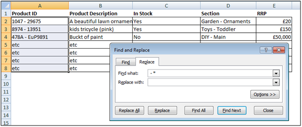
Find all characters including “ – “ and everything after it, and replace with nothing.
Note: In the example above I’ve had to highlight the column. If this wasn’t done first then it would find and replace this in the entire worksheet, including the data in column D.
- Now you want to grab the code before and the code after the dash, and store separately in two columns..
– Replicate the column entirely with copy and paste.
– On the first column, find “ – *” and replace with nothing.
– On the second column, find “* – “ and replace with nothing.
These tips should get you well on your way to using this great feature more productively. However, as a word of warning, make sure you are 100% confident in the data you are replacing. If I had a penny for every time I’ve seen people get into trouble with this feature.. well, I’d have quite a few pennies basically. Highlight data wherever possible to make sure you don’t apply it to the whole worksheet, and be very wary if you’re matching on just a few characters. For instance changing the misspell “ign” to “ing” on a huge list of keywords would also change “sign” and “resign” to “sing” and “resing”.
Best used: When you have massive spreadsheets and want to edit thousands of entries in a single command.
Stay tuned for more in my Excel series, including Excel formatting and advanced formulas. Make those presentations, forecasts and internal spreadsheets really shine and work for you and your business. We have an RSS so don’t delay in subscribing today!
Found is a London-based multi-award-winning digital growth, SEO, PPC, Social and Digital PR agency that harnesses the efficiencies of data and technology and future-thinking to help clients grow their businesses online.

